Episode 4: Visualizing Data
In this episode, you learn how to adjust data visualization in g.Pype.
Let’s begin with the code from the previous episode. Notice that the Generator constructor
is compact again, while the TimeSeriesScope constructor now includes three new parameters:
time_window, amplitude_limit, and hidden_channels, all set to their default values.
 1import gpype as gp
 2
 3if __name__ == "__main__":
 4
 5    app = gp.MainApp()
 6    p = gp.Pipeline()
 7
 8    source = gp.Generator(signal_amplitude=25)
 9
10    scope = gp.TimeSeriesScope(time_window=10,
11                               amplitude_limit=50,
12                               hidden_channels=[])
13
14    p.connect(source, scope)
15
16    app.add_widget(scope)
17
18    p.start()
19    app.run()  # blocking until window is closed
20    p.stop()
Again, first run the script to ensure the output is as expected.
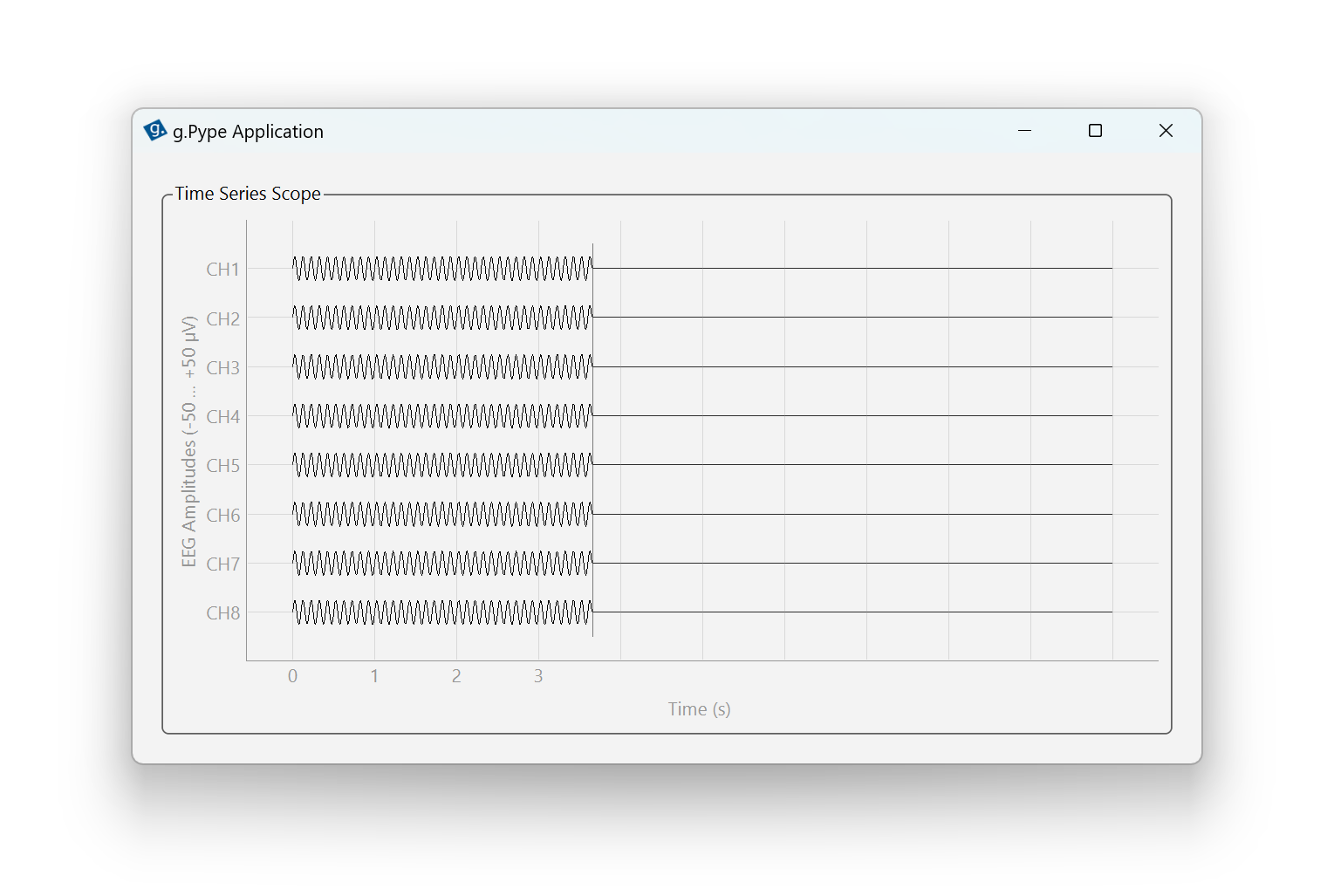
Figure 9: Minimal g.Pype application with a signal generator and time series scope.
Now, let’s customize the time TimeSeriesScope visualization using its parameters.
The time window determines how many seconds of data are displayed in the scope. By default, it’s 10 seconds.
Change the time window to 5 seconds by changing time_window=5 in the parameter list. Run the script
and observe that only 5 seconds of data are now visible. Let it run for a while to see how the scope
cursor overwrites older data. The x-axis automatically adjusts to the displayed segment.
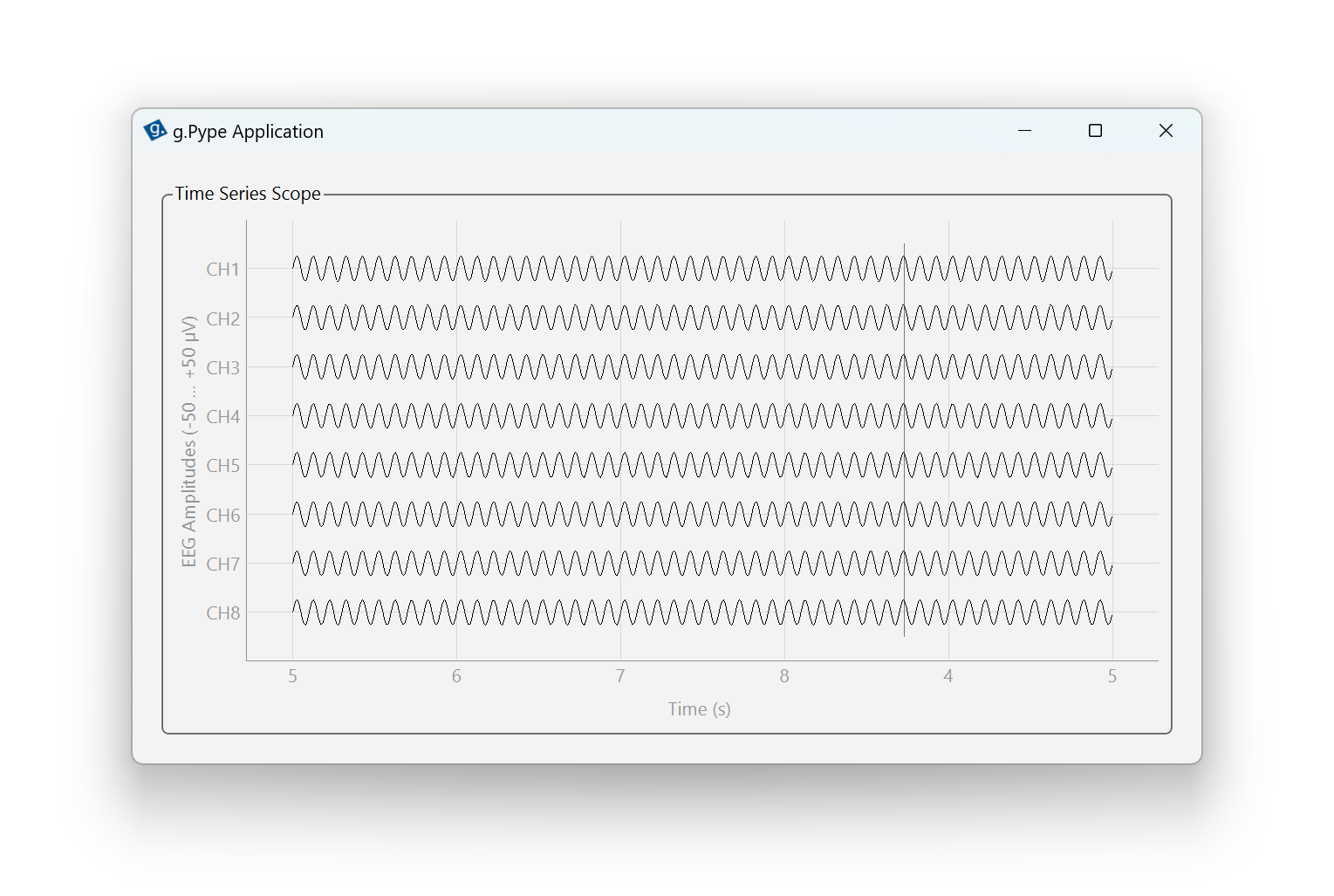
Figure 10: Time window reduced to 5 seconds.
The amplitude limit sets the y-axis range in microvolts (µV), controlling how much vertical space each channel receives.
By default, each channel is allocated 25 µV above and below its center line, for a total height of 50 µV per channel.
The scope’s grid lines are spaced accordingly, making it easy to estimate signal amplitudes. Change the amplitude limit to 25 µV
by changing amplitude_limit=25 in the parameter list. Run the script and notice how the sinusoids (with amplitude 25 µV)
now touch each other in the scope.

Figure 11: Amplitude limit set to 25 µV.
Sometimes, you may want to hide specific channels from the scope view, especially if you have many channels or want to focus on a subset.
For example, you might exclude trigger channels that aren’t relevant for your analysis. By default, all channels are shown.
To hide the first and last channel, set hidden_channels=[0, 7] in the parameter list (note: Python uses zero-based indexing).
Run the script and observe that only six channels are now displayed, with the channel labels reflecting that
channel 1 and 8 have been excluded.
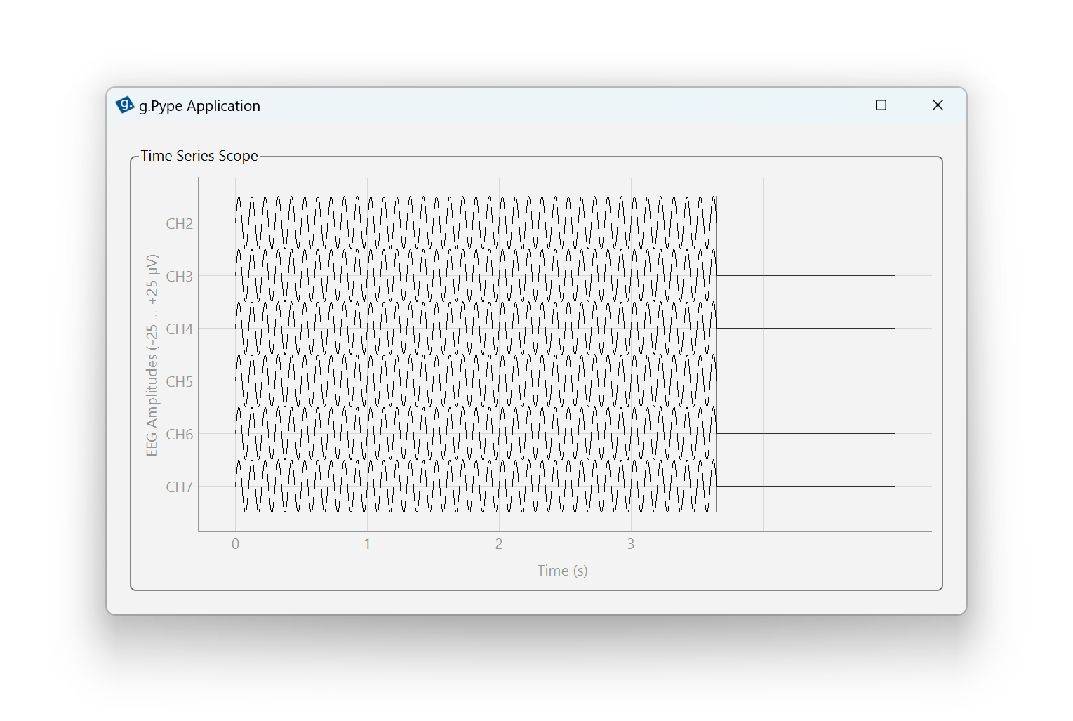
Figure 12: First and last channel hidden.
All set! You can now control TimeSeriesScope with its most important parameters to adjust the visualization to your needs.
In this episode, you learned how to adjust the TimeSeriesScope parameters to:
Change the time window
Set the amplitude limit
Hide specific channels
Note that there are additional parameters available for advanced use cases. We will cover them in upcoming episodes.
Now, you have successfully completed Season 1 of the g.Pype training. You are ready to proceed to Season 2, where we will discover g.Pype’s library building blocks for standard processing pipelines.
File s1e4_time_series_scope.py – View file on GitHub
 1# --------------------------------------------------------------
 2# Example file s1e4_time_series_scope.py
 3# For details and usage, see g.Pype Training Season 1, Episode 4
 4# --------------------------------------------------------------
 5
 6import gpype as gp
 7
 8if __name__ == "__main__":
 9
10    # Create main app and pipeline
11    app = gp.MainApp()
12    p = gp.Pipeline()
13
14    # Create signal source
15    source = gp.Generator(signal_amplitude=25)
16
17    # Create scope
18    scope = gp.TimeSeriesScope(time_window=10,
19                               amplitude_limit=50,
20                               hidden_channels=[])
21
22    # Connect nodes
23    p.connect(source, scope)
24
25    # Add widget to main app
26    app.add_widget(scope)
27
28    # Start pipeline and run application
29    p.start()
30    app.run()  # blocking until window is closed
31    p.stop()